Google Sheets: Complete Guide

Google Sheets terms

To fully understand how to use Google Sheets, you must be familiar with common terms that you will find on this software because sometimes errors and warnings may appear, and you know how to deal with them knowing these terms.

• Cell: Spreadsheets are made with lots of cells. That rectangular box resulted from a vertical column’s intersection, and a horizontal row is called a cell.
• Row: Rows are the horizontal lines of cells. Numbers represent them from 1 to infinite. Therefore you can have spreadsheets of the size you need.

• Column: Columns are the vertical series of cells. Each one of them is represented by a letter. Despite that, as the rows, they can also be infinite. After the letter Z, the letters start becoming AA, AB, AC, and so on.

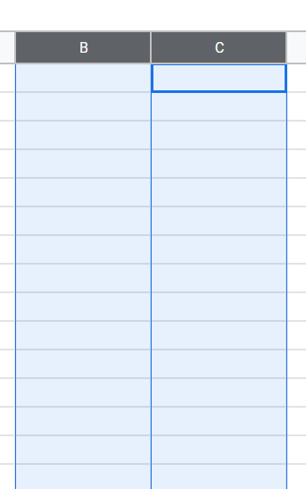
• Range: It is a group of selected cells. The range can be across a column, row, or both.

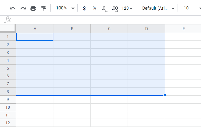
• Array: It is a range but used in a formula.
• Function: The operations that you can use to calculate values, and manage data. There is a function/formula bar between the spreadsheet grid and the toolbar. There is a function/formula bar (with the fx symbol). This space is used to type formulas, functions, text, etc.

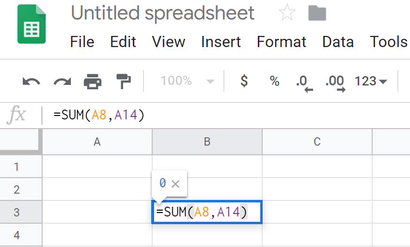
• Formula: To generate a result, we use formulas that combine functions, rows, cells, columns, and ranges.

How to Use Google Sheets the best way

After knowing the main terms of Google Sheets, it is time to learn how to use it properly. In fact, when you know each one of the elements, tools, and functionalities, you can improve your experience with this online software.

Toolbar

First things first, you need to be familiarized with the toolbar’s icons, so you can save time while editing your spreadsheets. This happens because you are taking shortcuts while using the toolbar directly, and not those infinite paths and clicks to get things done.

There are 28 tools available on the Sheets toolbar, and we are going to figure out each one of them:

• Undo: Represented by the curved arrow to the left helps correct any mistake you have made and restore immediate editions. 
• Redo: If you have undone something and want it back, click this button, represented by a curved arrow to the right.
• Print: Click on this symbol to print your spreadsheet. It’s a faster method than going to “File” then clicking on “Print.”
• Paint Format: If you want to easily set a format for your cells, select the cell or range of cells with the desired format. Then click on Paint Format to copy it. After this, the cursor will turn into a paint roller, and you can select the part of the spreadsheet you want to format.
• Zoom: It controls the size you display your document. For instance, when you need to see a cell in detail, you can zoom in to visualize it bigger.
• Format (as currency ($) and as a percentage(%): Ideal to format a range quickly with a currency or percentage.
• Decrease and Increase decimal places: Two buttons that can speed the process of changing the decimal position.
• More Formats: Here, you can see all the formats you can use in your data, including time, date, accounting, and others.
• Font: Choose the font style according to your needs.
• Font Size: Control the size of your font.
• Bold (B), Italic (I), Underline (U): Highlight your texts inside the spreadsheet with these styles
• Text Color: Change the color of your text to any existing color.
• Fill color: Fill your cells or ranges of cells with color. It’s a useful tool for tables because it facilitates viewing and organizing content.
• Borders: Choose how the borders will be, their color, and their style.
• Merge Cells: This tool only becomes available when you select a range. You can merge two or more cells.
• Align: You can align the data inside the cells to the left, center, or right.
• Vertical alignment: Align the position of your data to the top, center, or bottom of the cell.
• Text Wrapping: There are three possibilities for text wrapping inside Google Sheets (Overflow, Wrap, and Clip). They will basically help you display your text inside a cell or beyond the boundaries of a cell.
• Text Rotation: Sometimes, you need to display data differently. That is why this tool gives you the possibility of rotating the cell’s content from different angles.
• Insert Link: Select the word or sentence you want to be clickable and redirect to a certain URL. Then click on this symbol ( paper clip) and paste the URL in the popup.
• Insert comment: This is a useful tool for collaboration inside the spreadsheet. Select the cell or range you want to add a comment.
• Insert chart: If you work with charts, this button will be essential to you. Select the desired range of data you want to turn into a chart, then click on this button. A Chart Editor box will appear, and you will be able to set everything the way you need.
• Create a filter: A fast and easy way to start creating new filters.
• Functions: Here, you can see a drop-down list with the most used functions, such as SUM, AVERAGE, and COUNT. You can also choose from a list separated by categories (Math, Date, Engineering) or see all of them. This is helpful to insert the function, so you don’t need to memorize all of them.

How to Create a New Spreadsheet

To create a new spreadsheet, you have two options. The first one is to access the Google Sheets site and choose “Blank” represented by the plus symbol if you want to start from scratch. You can also choose a template to save you time, such as Invoices, Expense reports, monthly budgets, to-do lists.

And the list goes on and on with nice templates to help you with the design aspect of a spreadsheet. The other way is when you are already inside a spreadsheet and want to open a new one. Just click on “File,” then on “New” and “Spreadsheet.”

Protecting Your Data

Some sheets may have confidential data that needs to be protected. Google Sheets allows you to do that by following the steps:

Click on Data > Protected Sheets and Ranges.

• Then choose between Range to protect a specific range of cells or Sheet to protect the entire spreadsheet. If you choose the first one, select the range of cells you desire to protect.
• Next, click on Set Permissions, then choose to display a warning to those who intend to edit or customize editing permissions for certain people.

How to Hide and unhide Data

Additionally, you can protect your data by hiding it. Sometimes you need to restrict data views while sharing your spreadsheet, so Google Sheets also thought about adding this feature. To hide a column, click with the mouse’s right button on this column, and then select the option Hide Column.

Note that two arrows will appear in the columns between the one you hid. On the other hand, to unhide the column, hover over one of these arrows, then other arrows in a white box will appear. You can click on either of them to display the column again.

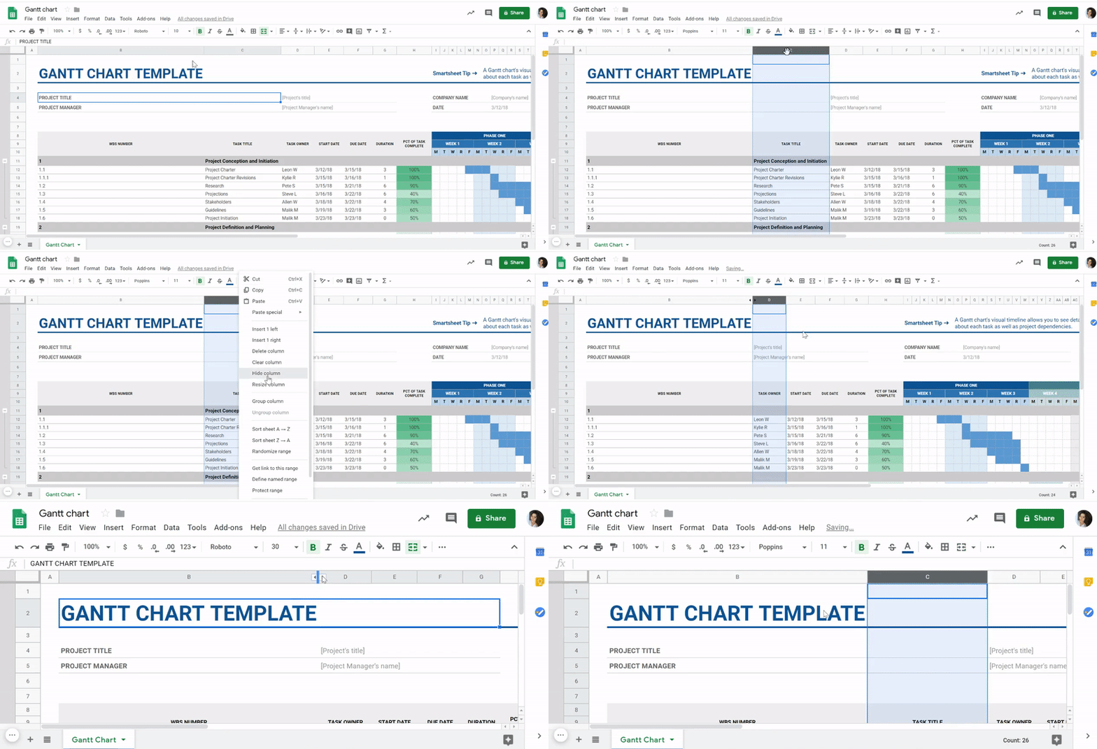
You can also use this resource when you want to control the data you are viewing at a time. As we said before, spreadsheets can have so much information that it is necessary to use some resources to view the content better. And this is one of the best resources.

Using filters to organize data

For starters, spreadsheets can have so much information that it may be hard to find what you need.

That’s why Google Sheets has numerous filters that will help you display only what you want to see. If you need to view data in a single column with specific criteria, for example, all the negative numbers on a table of financial content, you can apply a filter to do it. Or imagine you need to see all the cells that contain the industry your clients belong to, such as “Real Estate.”

To do the filtering process, start by selecting the column(s) you want to filter and then select Data on the menu bar. Then choose Create a Filter. Click on the funnel icon that will appear in the column, where you can choose to filter by value, condition, alpha, or numeric order.

This way, the spreadsheet will only show data that fits the criteria you have applied.

Edit Excel sheets in Google Sheets

Yes, you can edit Excel Sheets in the Google free software! Just import the file following this path: Go to “File,” then click on “Import,” choosing “Upload” next.

Please select the file you want to import, being aware that you must save it in file formats that don’t require password protection, such as .csv, .xls, and others. After that, the Excel sheet will be converted to a Google sheet.

Google Sheets advanced tips

Now that you are familiar with the basics of Google Sheets, how about level up and start learning more advanced tips?

Macros

This feature offers the possibility to store a command sequence or function on a VBA module. Therefore you can use it to perform a task, like a shortcut. It’s commonly used for repetitive tasks to avoid loss of time and long processes. Start creating your macros by going to Tools, then Macros.

Choose the option Record macro, manage, or import the existing ones.

Array Formulas

According to Google, an array formula is a formula that can perform multiple calculations on one or more items in an array. It’s a way to make the calculation inside your spreadsheet more efficient, mainly when it has a huge amount of data.

Check some examples of array formulas below:

Creating graphs

Displaying data in charts is one of the most used tools in the business context. That is the reason why it is so important to learn how to create them inside Google Sheets.

Go through the following steps:

1. Select the range of data you desire to transform in a chart. If you want to pre-label the chart, add a header row or column.
2. Next, click on “Insert,” then on “Chart.”
3. A side panel will open, then you have to choose the option “Data,” which is under “Chart type.” Next, choose a chart.
4. To personalize your chart style, text, and colors, click on “Customize.”

How to Create a Pivot Table

A Pivot Table is an advanced tool to calculate, summarize, and analyze data. It allows you to see patterns, trends, and comparisons in your data.

Follow these steps to create your pivot table in Google Sheets:

1. First, select the cells with data you want to use in your pivot table. Notice that each column needs a header.
2. Next, click on Insert in the menu bar and choose the Pivot table. Then click the pivot table sheet if it’s not open yet.
3. In the side panel, next to “Rows” or “Columns,” click “Add” and choose a value. To add an existing pivot table, under “Suggested,” select it.
4. Still in the side panel, click “Add” next to “Values.” After, choose the value you desire to display in your rows or columns.
5. If you want to change something, click the down arrow next to it.

Translate without leaving your Google Sheet

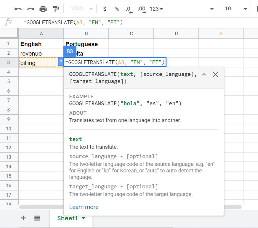
If you need to work with Sheets in another language, you can save time by using this function: GOOGLETRANSLATE. It will translate all values into a different language.

10 Google Sheets Formulas you should know

Many times you need to get quick results inside a spreadsheet. That’s why people use formulas for almost everything. It facilitates your work one hundred percent because you don’t need to worry about calculating by yourself.

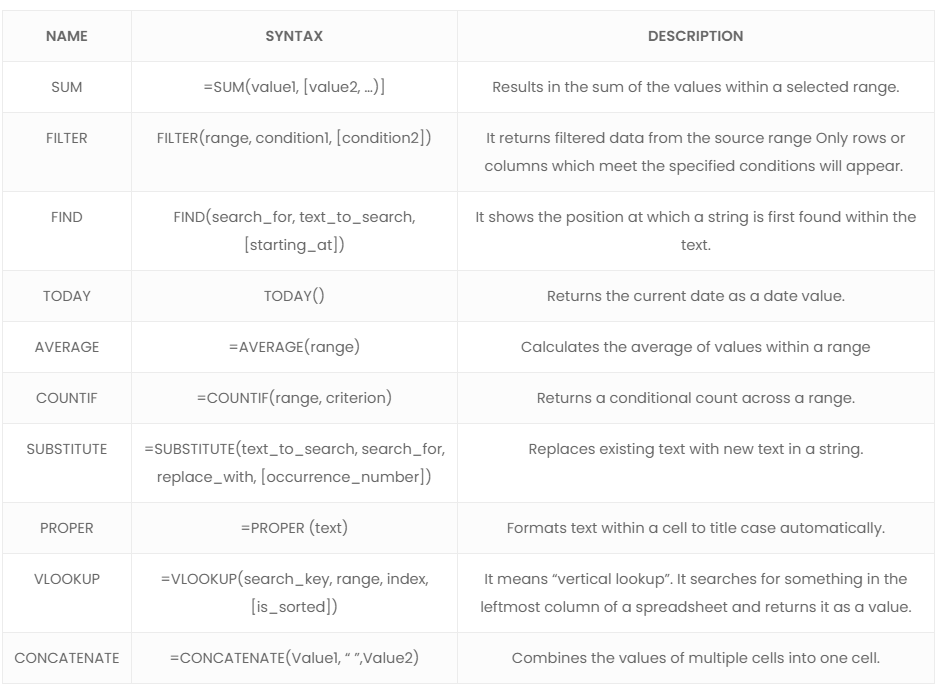
So check the 10 most commonly used Google Sheets formulas, and learn how to deal with your data the best way possible.
There are lots of formulas you can use besides these. Check them out on the Google Sheets function list. They are divided into categories: Array, Database, Date, Engineering, Filter, Financial, Google, Info, Logical, Lookup, Math, Operator, Statistical, Text, Parser, and web.

Google Sheets FAQs

How do I collaborate with others on a Google Sheet?

Google Sheets makes real-time collaboration easy:

Sharing the Sheet:

• Click the green “Share” button at the top-right corner.
• Enter email addresses of collaborators.
• Set permissions (View, Comment, or Edit).

Real-Time Collaboration Tools:

• Chat: Use the built-in chat feature when multiple users are editing simultaneously.
• Comments & Task Assignments: Add comments or assign tasks by selecting a cell, clicking “Add comment,” and tagging collaborators with +email.

Email Collaborators:

• Go to File > Email Collaborators to send updates or questions directly from the sheet.

Can I import data from other sources into Google Sheets?

Yes, you can import data from various sources:

From Other Google Sheets:

• Use the IMPORTRANGE function to pull data from another spreadsheet.

From CSV or Excel Files:

• Go to File > Import, upload your file, and choose how to integrate it (e.g., replace or append data).

From Web Sources:

• IMPORTHTML: For tables or lists on web pages.
• IMPORTXML: For structured web data via XPath queries.
• IMPORTDATA: For CSV or TSV files hosted online.

What are the best practices for organizing data in Google Sheets?

To keep your data clean and manageable:

• Use Clear Headers: Label columns clearly to describe their content (e.g., “Name,” “Date,” “Amount”).
• Sort and Filter Data:
  • Sort alphabetically, numerically, or by date using the Data > Sort range option.
  • Apply filters (Data > Create a filter) to view specific subsets of data.
• Group Rows/Columns: Right-click on rows/columns and select “Group” for hierarchical organization.
• Apply Conditional Formatting: Highlight trends or outliers automatically based on rules.
• Use Separate Sheets for Different Data Types: Keep raw data, calculations, and summaries in distinct sheets within the same file.